T1 and Ramsey
Two coherence measurements that differ by two lines of program. T1 puts the qubit in its excited state, idles for a delay, and reads out; repeating that over a range of delays gives the exponential whose time constant is the energy relaxation time. Ramsey replaces the single pi pulse with two pi/2 pulses around the same idle and advances the phase of the second one in proportion to the delay, so the population oscillates at a frequency you chose and decays under an envelope you did not. Both are on the calibration ladder immediately after Rabi, because both need a pi pulse that Rabi is what calibrates.
These are the first programs on these pages with a time axis. Rabi sweeps an amplitude and the CZ chevron sweeps a waveform parameter; neither sweeps a duration, which is where wait comes in. Along with it come the two operations that move an oscillator's phase, reset_phase and set_phase, and the measurement field that reports a classified outcome instead of an IQ point.
The T1 program
import qprogram as qp

schema = qp.BusSchema.transmon()
q = schema.q

t1 = qp.QProgram(
    label="t1",
    description="Energy relaxation on q0",
    schema=schema,
)
delay = t1.variable("delay", label="Delay", units="ns")

with t1.average(shots=1000):
    with t1.sweep(delay, qp.Linspace(0.0, 40_000.0, num=41)):
        t1.play(q[0].drive, "pi_pulse")
        t1.wait(q[0].drive, delay)
        t1.sync()
        m0 = t1.measure(
            q[0].readout,
            "readout",
            "weights",
            fields=(qp.MeasurementField.IQ, qp.MeasurementField.STATE),
        )
Why each piece is where it is
wait(bus, duration) idles one bus for a number of nanoseconds and takes either an integer or an Expression, so the loop variable goes straight in. It idles a bus rather than the program, which is why the sync() that follows is what makes the delay reach the readout: the wait pushes the drive bus forward in time, and the sync brings every other bus up to it before the measurement starts. Waiting on q[0].readout instead and syncing would express the same experiment; waiting on neither would measure at a fixed time after the pulse no matter what delay held.
Nothing checks the duration at the call site. wait(q[0].drive, 17) and wait(q[0].drive, 3.5) both build, even though a sequencer with a 4 ns time grid can run neither. Duration limits belong to the platform, and qp.validate reports them against the bus slot's min_wait_duration_ns; see Capabilities, diagnostics, and profiles.
Asking for MeasurementField.STATE alongside IQ records the classified outcome as well as the point it was classified from. It is the field a relaxation curve is read off, because what T1 measures is a population rather than a position in the IQ plane. Requesting a field is a decision made where the measurement is built, not where the result is read, so a field left out here cannot be recovered from the result later.
The delays run to 40 microseconds in 41 points, which is a range set by the device rather than by the language: it wants to cover roughly three relaxation times so that the tail is flat enough to fit a baseline against.
What it produces
#!QProgram 0.2

metadata:
  label: "t1"
  description: "Energy relaxation on q0"

schema:
  element q:
    drive info=IQ
    readout info=IQ+acquires

body:
  var delay label="Delay" units="ns"

  average 1000:
    for delay in Linspace(start=0.0, stop=40000.0, num=41):
      play q[0].drive "pi_pulse"
      wait q[0].drive delay
      sync
      measure q[0].readout "readout" "weights" name="q0/readout/m0" fields=["state", "iq"]
The fields= list is written in the format's own order rather than the order the call passed, so (IQ, STATE) and (STATE, IQ) produce the same file. A measurement that asks only for the default IQ omits the attribute entirely, which is why neither the Rabi program nor the chevron has one.
The Ramsey program
The skeleton is the same. What changes is the pulse pair around the wait and the phase written between them:
import numpy as np

ramsey = qp.QProgram(
    label="ramsey",
    description="Ramsey fringes on q0",
    schema=schema,
)
delay = ramsey.variable("delay", label="Free evolution", units="ns")

with ramsey.average(shots=1000):
    with ramsey.sweep(delay, qp.Linspace(0.0, 3000.0, num=151)):
        ramsey.reset_phase(q[0].drive)
        ramsey.play(q[0].drive, "pi_half")
        ramsey.wait(q[0].drive, delay)
        ramsey.set_phase(q[0].drive, 2 * np.pi * 2e-3 * delay)
        ramsey.play(q[0].drive, "pi_half")
        ramsey.sync()
        m1 = ramsey.measure(
            q[0].readout,
            "readout",
            "weights",
            fields=(qp.MeasurementField.IQ, qp.MeasurementField.STATE),
        )
The first pi/2 pulse puts the qubit on the equator, the wait lets it precess, and the second one turns that accumulated phase into a population the readout can see. set_phase before the second pulse advances the reference frame by 2 pi times 2 MHz times the delay, which makes the fringe oscillate at 2 MHz whether or not the drive is on resonance. That artificial detuning is the point of the line: a Ramsey run at zero detuning decays without oscillating, and a slow decay does not say how far off the drive frequency is or in which direction, while a 2 MHz fringe does both and leaves the decay envelope separable from the frequency error.
set_phase is absolute and takes radians. There is no operation that shifts the phase by an increment, so a sequence that wants to accumulate phase computes the total itself, which is what the multiplication by delay does here. reset_phase at the top of the body is what makes that total meaningful: it zeroes the oscillator's phase so every iteration starts from the same reference instead of from wherever the previous iteration left it.
The phase expression serializes as a single product:
Three of the four factors were plain Python floats, so Python multiplied them before the DSL was handed the result. Only the factor that touches a variable survives as a node, which is the same folding the fine scan on the Qubit spectroscopy page relies on. The cost is that set_phase now asks a platform for expr.binary_op and expr.constant on top of op.set_phase and expr.variable.
Reading the results
Both programs are resolved against the same calibration set and run the same way. What differs is the model, since the executor simulates no timing at all and therefore no relaxation:
library = {
    "pi_pulse": qp.waveforms.IQDrag(amplitude=0.5, duration=40, sigma=8, beta=0.1),
    "pi_half": qp.waveforms.IQDrag(amplitude=0.25, duration=40, sigma=8, beta=0.1),
    "readout": qp.waveforms.IQPair(qp.waveforms.Square(1.0, 2000), qp.waveforms.Square(0.0, 2000)),
    "weights": qp.waveforms.IQPair(qp.waveforms.Square(1.0, 2000), qp.waveforms.Square(1.0, 2000)),
}

result = qp.simulate(
    t1.with_waveforms(library),
    model=qp.MockMeasurementModel(
        p_excited=lambda bus, env: float(np.exp(-env["delay"] / 12_000.0)),
        seed=3,
    ),
)

population = result.get(m0, field=qp.MeasurementField.STATE)
population.dims  # ("delay",)
population.shape  # (41,)
population.coords["delay"]  # 0.0, 1000.0, ..., 40000.0
p_excited is the second callback qp.MockMeasurementModel takes. Where response returns the noiseless IQ point, p_excited returns the probability that a shot classifies as excited, and the executor draws a Bernoulli sample from it per shot. Both receive the same (bus, env) pair, so a decay written against env["delay"] is all it takes to give the curve a shape. Without a p_excited argument every shot classifies as 0.
The curve is the exponential the model was given, sampled a thousand shots per point, and the scatter around it is the Bernoulli noise of that count. delay was declared in nanoseconds and runs to 40000, which is not how anyone reads a T1, so the figure restates it:
result.plot(
    m0,
    field=qp.MeasurementField.STATE,
    coords={"delay": qp.plotting.Quantity(units="μs", transform=lambda v: v / 1000)},
    value=qp.plotting.Quantity("Excited-state population"),
    style=qp.plotting.Style(markers=True),
)
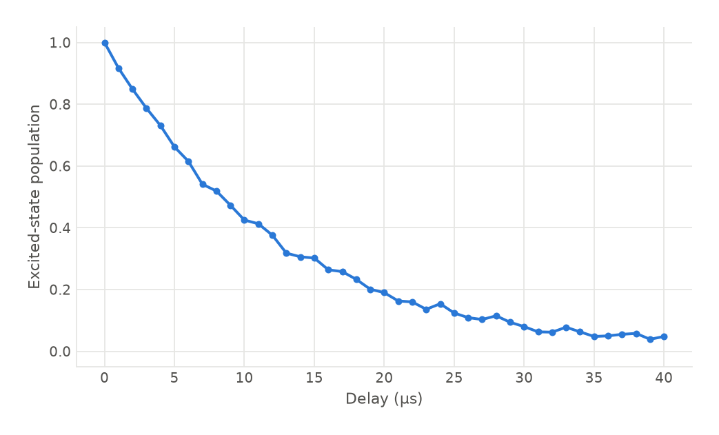
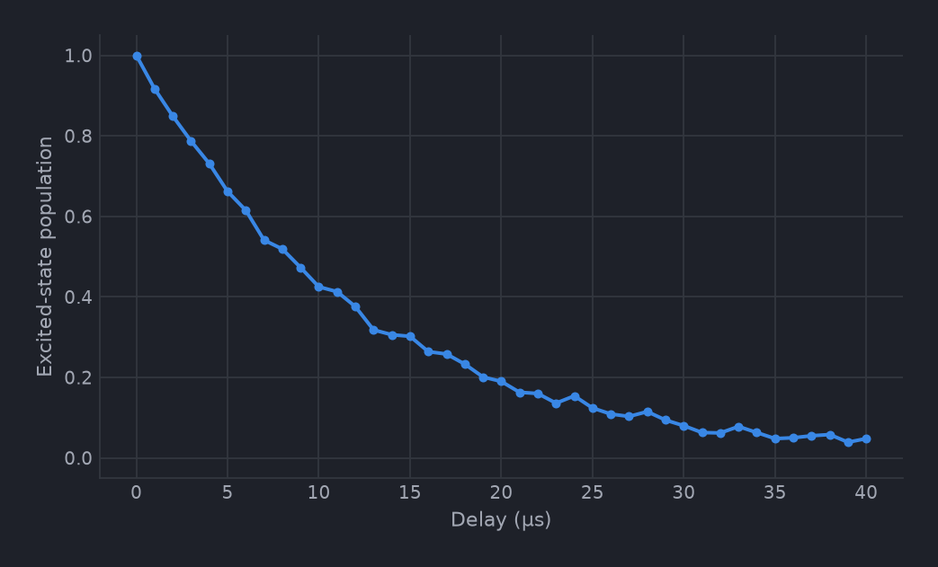
The label the variable was given survives the restatement and only the unit moves, so the axis reads Delay (μs). markers=True earns its place on a 41-point sweep, where the points are the measurement and the line between them is interpolation. Plotting results covers the rest.
The STATE array has no trailing "IQ" dimension, because a classified outcome is one number per shot rather than a pair. result.get(m0) on the same handle still returns the IQ field with dims ("delay", "IQ") and shape (41, 2). This is the mirror of the raw trace on the Rabi page: a RAW field adds a "time" dimension in front of "IQ", and a STATE field takes "IQ" away.
Under an averaging block the values are the mean of those Bernoulli draws, so each point is the excited-state population at that delay rather than a single 0 or 1. They carry the sampling noise of the shot count that produced them, which is the honest reason a T1 fit wants a thousand shots per point and not fifty.
Ramsey reads back identically, with a model that oscillates as well as decays:
def fringe(bus, env):
    """2 MHz fringe under a 1.5 microsecond envelope."""
    t = env["delay"]
    return 0.5 * (1 - np.cos(2 * np.pi * 2e-3 * t) * np.exp(-t / 1500.0))


result = qp.simulate(
    ramsey.with_waveforms(library),
    model=qp.MockMeasurementModel(p_excited=fringe, seed=1),
)
result.get(m1, field=qp.MeasurementField.STATE).dims  # ("delay",)
The 20 ns spacing that Linspace(0.0, 3000.0, num=151) resolves to samples the 2 MHz fringe 25 times per period, which is the constraint that sets the point count: the delay axis has to resolve the artificial detuning, not just reach far enough to see the envelope.
The fringe and the envelope are the two things the measurement separates. The oscillation is the 2 MHz the program put there; the decay it sits inside is the one the qubit contributed:
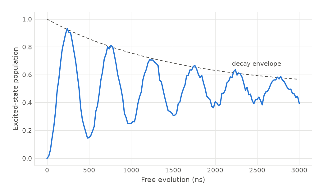
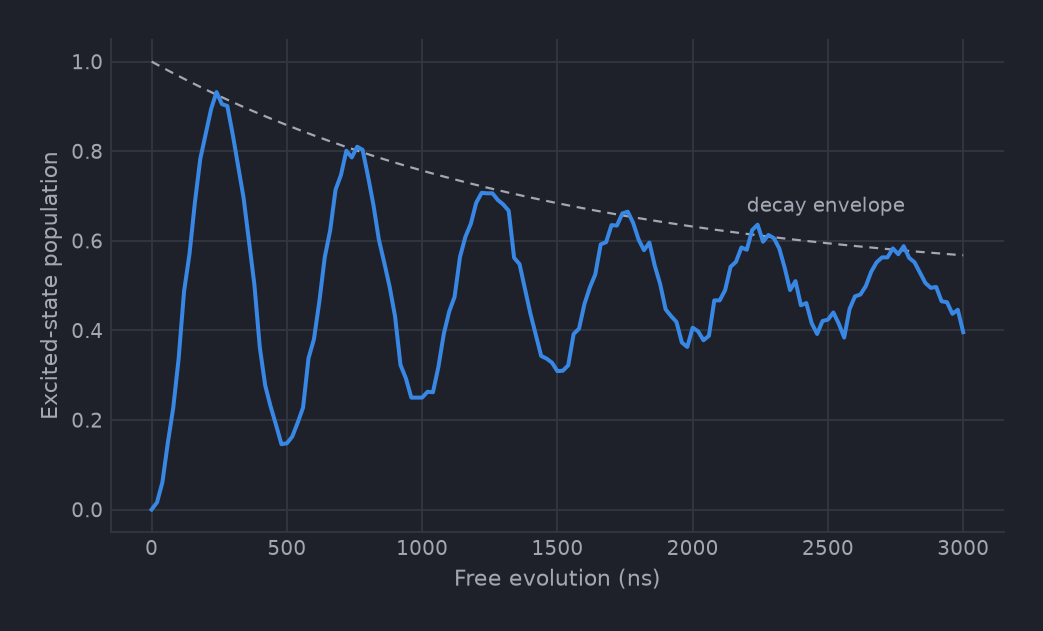
Nothing in either run knows about relaxation or precession. wait evaluates its expression and returns, set_phase and reset_phase do the same, and the curves come entirely from the two model callbacks reading env["delay"]. See Running programs for what the reference executor does and does not simulate.
Adapting it
A Hahn echo measures T2 instead of T2 star by putting a pi pulse in the middle of the idle, which refocuses the dephasing that is static over one shot. The delay is then split in half on either side of it:
half = delay / 2
echo.play(q[0].drive, "pi_half")
echo.wait(q[0].drive, half)
echo.play(q[0].drive, "pi_pulse")
echo.wait(q[0].drive, half)
echo.play(q[0].drive, "pi_half")
delay / 2 is an expression like any other and appears in the file as (delay / 2). Extending it to a CPMG train means repeating the middle pair n times, and a Python for loop around those two lines writes n copies into the program at build time rather than a loop into the file. When n is large enough for that to be unwieldy, a fragment names the repeated piece once.
To space the delays logarithmically, which puts points where an exponential actually curves, swap the source for qp.Logspace(100.0, 40_000.0, num=41). Its bounds are linear values spaced evenly on a log scale, and both must be positive, so a T1 axis written this way cannot start at zero the way the Linspace above does.
To find the qubit frequency from the Ramsey rather than from a spectroscopy scan, run it twice with the artificial detuning at plus and minus 2 MHz. The fringe frequency that comes back is the sum of the artificial detuning and the real error, so the two runs separate the error's magnitude from its sign, which a single run cannot do.
To read the fringe as an IQ trajectory instead of a population, drop MeasurementField.STATE from fields= and plot data.sel(IQ="I") against data.sel(IQ="Q"). That form needs no classifier on the instrument, which matters on a platform whose readout chain cannot discriminate states in real time. See Measurements and results.