CZ chevron
A CZ chevron is a two-axis sweep used to calibrate a two-qubit gate. You prepare a state, fire a flux pulse whose amplitude and duration both vary, and read the qubits out. The interference fringes in the resulting heatmap converge on the amplitude where the two qubits are resonant, which is the chevron's tip and the point the gate is tuned to.
Three things appear here that the Rabi example does not have: a schema with a single-channel flux bus, two nested sweeps, and an inline waveform whose parameters are the sweep variables.
The program
import qprogram as qp

schema = qp.BusSchema.flux_tunable_transmon()
q = schema.q

program = qp.QProgram(
    label="cz_chevron",
    description="Sweep flux amplitude and duration to map the CZ chevron",
    schema=schema,
)
amp = program.variable("amp", label="Flux amplitude", units="V")
dur = program.variable("dur", label="Flux duration", units="ns")

with program.average(shots=1000):
    with program.sweep(amp, qp.Range(0.0, 1.0, 0.01)):
        with program.sweep(dur, qp.Range(10, 210, 2)):
            # Prepare q1 in |1>.
            program.play(q[1].drive, "pi")
            program.sync()

            # Apply the flux pulse with sweeping amplitude and duration.
            program.play(
                q[0].flux,
                qp.waveforms.FlatTop(amplitude=amp, duration=dur, smooth_duration=5),
            )
            program.sync()

            # Read out both qubits.
            m0 = program.measure(q[0].readout, "readout", "weights")
            m1 = program.measure(q[1].readout, "readout", "weights")
Why each piece is where it is
qp.BusSchema.flux_tunable_transmon() gives element q three bus kinds: drive (IQ), readout (IQ, with an ADC), and flux (single channel). The channel type is enforced at the call site, so a Play of an IQ waveform on q[0].flux raises ValidationError: Bus 'q0/flux' is a single channel but received an IQWaveform (IQDrag) when the program is built rather than when a compiler runs.
The two sweeps are nested with amp outside and dur inside, so the flux pulse visits every (amp, dur) pair, which is the grid a chevron pattern lives on. Nesting order decides two things at once: the inner variable moves fastest during execution, and the result dimensions come back in nesting order, outermost first. Each qp.Range holds round((stop - start) / step) + 1 points, so Range(0.0, 1.0, 0.01) is 101 amplitudes and Range(10, 210, 2) is 101 durations, for 10201 grid points.
FlatTop(amplitude=amp, duration=dur, smooth_duration=5) stores the two variables as parameters of the waveform node. Nothing materializes the sweep at build time; the platform decides whether to update an amplitude register, regenerate the envelope per point, or refuse the program because its compiler cannot do either. The reference executor renders no envelope at all, so it accepts the program either way and tells you nothing about whether real hardware would.
smooth_duration=5 sets the length of each erf-shaped edge, and duration counts the edges in rather than adding them. The rise crosses half amplitude 5 ns in and is flat to within a part in 10⁵ by 10 ns, so the shortest few durations on the axis, where dur is not comfortably above 2 * smooth_duration, never reach full amplitude at all. That is a property of the pulse shape rather than of the sweep, and it is what makes the near edge of the duration axis worth reading with care.
The pi pulse plays on q[1].drive while the flux pulse plays on q[0].flux, and the sync() between them is what stops the flux pulse from starting before the preparation is over. The second sync() does the same for the readout.
m0 and m1 are two handles on the same shot. Auto-allocated names carry a per-bus counter, so both come out as m0 under different bus prefixes: q0/readout/m0 and q1/readout/m0.
What it looks like on disk
#!QProgram 0.2

metadata:
  label: "cz_chevron"
  description: "Sweep flux amplitude and duration to map the CZ chevron"

schema:
  element q:
    drive info=IQ
    readout info=IQ+acquires
    flux info=single

body:
  var amp label="Flux amplitude" units="V"
  var dur label="Flux duration" units="ns"

  average 1000:
    for amp in Range(start=0.0, stop=1.0, step=0.01):
      for dur in Range(start=10.0, stop=210.0, step=2.0):
        play q[1].drive "pi"
        sync
        play q[0].flux FlatTop(amplitude=amp, duration=dur, smooth_duration=5, buffer=0)
        sync
        measure q[0].readout "readout" "weights" name="q0/readout/m0"
        measure q[1].readout "readout" "weights" name="q1/readout/m0"
FlatTop's buffer argument defaults to 0 and was not passed, but the writer spells out every constructor argument so that reading the file back rebuilds the same waveform without depending on today's defaults. Range's integer bounds come back as 10.0 and 210.0 because a source stores its bounds as floats. Sweep variables inside a waveform are written as bare identifiers, and the parser resolves them against the var declarations above.
Reading the results
The reference executor is an interpreter that walks every shot of every grid point, so its cost is the product of the axes. At the sizes above that is 101 amplitudes by 101 durations by 1000 shots by 2 measurements, which is 20.4 million model samples and minutes of wall clock on one core; an 11 by 11 grid at the same shot count is 84 times less work and returns in seconds. Coarsen the steps or lower average(shots=...) while you are iterating: the dimensions and coordinates below come back the same either way, only shorter.
import numpy as np

library = {
    "pi": qp.waveforms.IQDrag(amplitude=0.5, duration=40, sigma=8, beta=0.1),
    "readout": qp.waveforms.IQPair(qp.waveforms.Square(1.0, 2000), qp.waveforms.Square(0.0, 2000)),
    "weights": qp.waveforms.IQPair(qp.waveforms.Square(1.0, 2000), qp.waveforms.Square(1.0, 2000)),
}


def chevron(bus, env):
    """A two-level model of the swap: population against detuning and time."""
    coupling = 0.01  # 1/ns
    detuning = 0.05 * (env["amp"] - 0.5)  # zero at the interaction point
    rate = np.hypot(coupling, detuning)
    return (coupling / rate) ** 2 * np.sin(np.pi * rate * env["dur"]) ** 2 + 0j


result = qp.simulate(
    program.with_waveforms(library),
    model=qp.MockMeasurementModel(response=chevron),
)

data0 = result.get(m0)
data1 = result.get(m1)

# One dimension per enclosing sweep, outermost first.
data0.dims  # ("amp", "dur", "IQ")
data0.shape  # (101, 101, 2)
data0.coords["amp"]  # 0.00, 0.01, ..., 1.00
data0.coords["dur"]  # 10.0, 12.0, ..., 210.0
data1 is the same grid measured on q[1].readout and has identical dims and shape, since both measurements sit under the same two sweeps. Reading both is what separates population moving from q1 to q0 from population being lost, which a single readout cannot tell apart.
The response function receives the currently bound loop variables by id, so env["amp"] and env["dur"] are the coordinates of the grid point being measured. It is called once per shot per measurement, and bus is the bus string, so a model can respond differently on q0/readout and q1/readout. Without a model= argument, qp.simulate uses a qp.MockMeasurementModel that responds 0j everywhere and the heatmap is flat zero. The model above is a stand-in for physics, not a simulation of the chip: it exists so the plot below has a chevron in it.
average contributes no dimension, so the shots are already averaged out of data0 when you get it: the executor sums per grid point and divides by the shot count it recorded there. A grid point holds NaN when that count is zero, which happens only for a measurement inside a conditional arm the program never selected at that point.
Two swept dimensions besides IQ give a heatmap, and the array is already on the grid, so no reshaping is needed. A heatmap colours one surface, so name the quadrature you want; leaving channels out takes the magnitude instead:
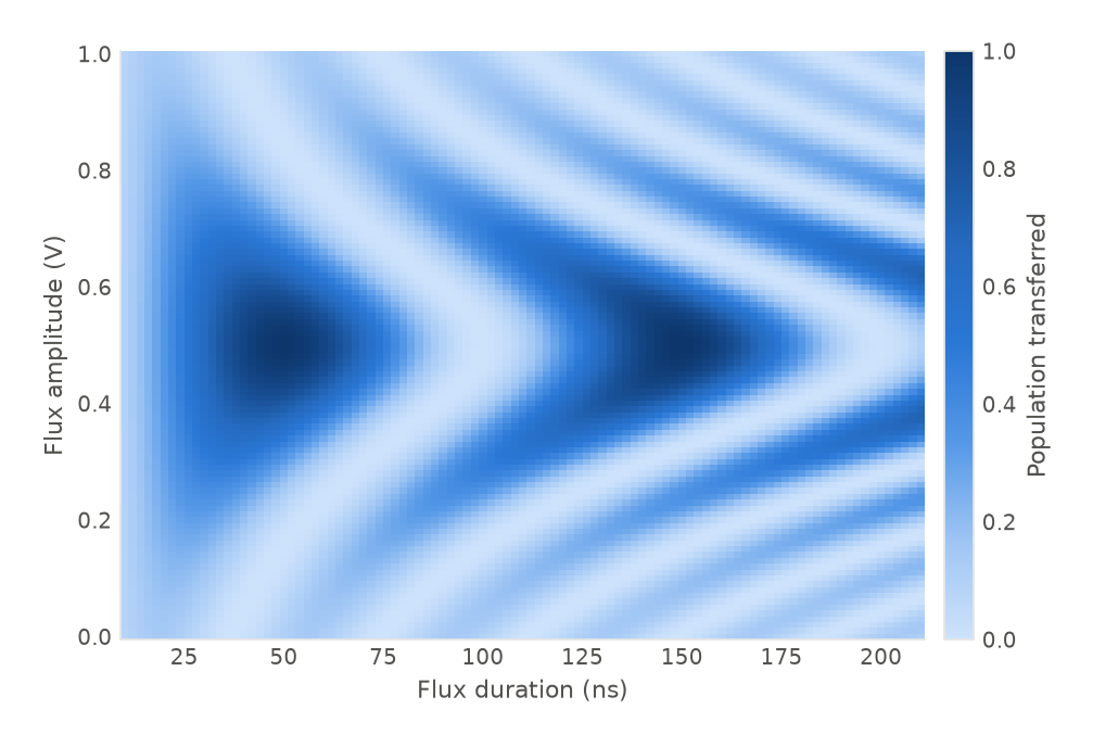
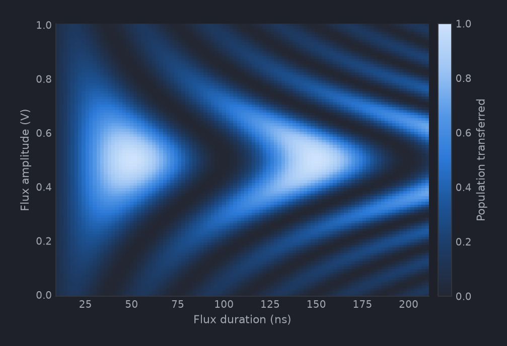
The inner sweep runs along the x axis and the outer one up the y axis, matching the loop nesting rather than the dimension order in data0.dims; x= and y= say otherwise. matplotlib is not a runtime dependency; it comes with the viz extra, installed with pip install "qprogram[viz]". Plotting results covers the rest.
Adapting it
To move both parameters together, taking one diagonal cut through the grid instead of the whole grid, compose the loops in parallel rather than nesting them:
The two sources must then hold the same number of points, and both do here at
101. When they do not, the composition is rejected as it is built: ValidationError: parallel loops must have the same number of iterations to advance in lockstep; got Sweep('amp'): 11, Sweep('dur'): 12. The results come back on one "amp|dur" dimension of 101 points carrying amp and dur as coordinates along it, which plot draws as one axis with the other above it. See Control flow.
For the SNZ flavor of CZ, swap the waveform and leave the rest of the program alone:
SuddenNetZero is a positive square segment, a zero hold of t_phi ns, then a negative segment scaled by b, all inside duration. It is single channel like FlatTop, so the bus check passes unchanged, and b is the parameter you detune from 1 to null whatever residual flux the line adds.
If the chip has dedicated couplers, use qp.BusSchema.flux_tunable_transmon_coupled() and drive schema.c[0, 1].flux instead of q[0].flux. A coupler index is a tuple, and the resolved bus name joins it with an underscore, giving c0_1/flux. See Buses and schemas.
To keep the raw ADC trace alongside the IQ point, request it per measurement with fields=(qp.MeasurementField.IQ, qp.MeasurementField.RAW) and read it back with result.get(m0, field=qp.MeasurementField.RAW), which adds a "time" dimension between the sweeps and "IQ". On a 101 by 101 grid that is a large array, so it is worth coarsening the sweeps first. See Measurements and results.