CPMG on two qubits
A CPMG sequence puts a train of refocusing pi pulses between two pi/2 pulses. Each pi pulse reverses the phase the qubit has accumulated since the last one, so noise slower than the pulse spacing cancels and noise faster than it does not, which makes the measured coherence time a function of the spacing and the train a filter you can tune. Sweeping the spacing and reading the surviving coherence is how the noise spectrum of a qubit is measured.
Written out, the sequence is the same three lines repeated as many times as the train is long, once per qubit. This page writes them once. A Fragment is a named, parameterized sub-program, and program.call appends a reference to it rather than a copy, so the file holds one definition and one line per call site. Fragments covers the mechanism in full; what follows is an experiment that needs one.
The program
import numpy as np
import qprogram as qp

schema = qp.BusSchema.transmon()
q = schema.q


@qp.fragment
def cpmg(f, drive, readout, tau):
    """Two pi/2 pulses around a train of four refocusing pi pulses."""
    f.play(drive, "pi_half")
    for _ in range(4):
        f.wait(drive, tau / 2)
        f.play(drive, "pi")
        f.wait(drive, tau / 2)
    f.play(drive, "pi_half")
    f.sync([drive, readout])
    f.measure(readout, "readout", "weights", fields=(qp.MeasurementField.STATE,))


program = qp.QProgram(
    label="cpmg",
    description="CPMG coherence on q0 and q1",
    schema=schema,
)
tau = program.variable("tau", label="Pulse spacing", units="ns")

with program.average(shots=1000):
    with program.sweep(tau, qp.Linspace(20.0, 2000.0, num=100)):
        program.call(cpmg, q[0].drive, q[0].readout, tau)
        program.call(cpmg, q[1].drive, q[1].readout, tau)
Why each piece is where it is
The decorated name is the fragment. After @qp.fragment runs, cpmg is a qp.Fragment instance rather than a function, and calling it directly is not how it is used; program.call(cpmg, ...) is. The first parameter receives the fragment's own builder, which is why the body writes f.play rather than program.play, and every parameter after it becomes a qp.Parameter bound at the call site. The fragment's name comes from __name__.
The three bindings are of three different kinds. drive and readout are bound to buses, tau to an expression. Parameters are untyped and it is the binding that decides, checked when the call is expanded, so a bus passed where an expression is expected is caught then rather than at the call site.
tau / 2 works because qp.Parameter subclasses qp.Variable, so a parameter participates in expressions exactly as a swept variable does. Half the spacing falls on each side of every pi pulse, which is what makes the refocusing symmetric.
sync([drive, readout]) names its buses instead of taking the argument-free form, which would align every bus the program has touched and couple the two qubits to each other. Naming them keeps each call closing only its own train before its own readout, so the two trains are independent and an instrument is free to run them at the same time.
What it produces
#!QProgram 0.2

metadata:
  label: "cpmg"
  description: "CPMG coherence on q0 and q1"

schema:
  element q:
    drive info=IQ
    readout info=IQ+acquires

fragment cpmg(drive, readout, tau):
  play drive "pi_half"
  wait drive (tau / 2)
  play drive "pi"
  wait drive (tau / 2)
  wait drive (tau / 2)
  play drive "pi"
  wait drive (tau / 2)
  wait drive (tau / 2)
  play drive "pi"
  wait drive (tau / 2)
  wait drive (tau / 2)
  play drive "pi"
  wait drive (tau / 2)
  play drive "pi_half"
  sync drive readout
  measure readout "readout" "weights" name="m0" fields=["state"]

body:
  var tau label="Pulse spacing" units="ns"

  average 1000:
    for tau in Linspace(start=20.0, stop=2000.0, num=100):
      cpmg(q[0].drive, q[0].readout, tau)
      cpmg(q[1].drive, q[1].readout, tau)
The Python for _ in range(4) is nowhere in that file. A fragment body runs once, at decoration time, to record its AST, so the loop executed then and wrote four copies of its three statements into the fragment. Python control flow inside a fragment body is a code generator, not a runtime construct, and the twelve lines above are what it generated.
That is also the limit of it. Because the count is resolved at decoration, n cannot be a parameter: a train of eight needs a second fragment or a range(n) closed over at definition time, and either way each length is a distinct definition in the file. The parameters are the things that vary per call site, and the structure is not one of them.
Bus arguments write as bare identifiers inside the definition (play drive, not a bus path) because they are parameters there, and the call statements carry the real buses. The measurement's auto-allocated name is m0 with no bus prefix for the same reason: at definition time there is no bus to derive a prefix from.
Getting the handles back
program.call returns None. The measurement is inside the fragment, so nothing at the call site hands back a qp.MeasurementHandle, and the program does not yet know how many measurements it has:
expand() returns a copy with every Call inlined, and the handles appear on it:
flat = program.expand()
[h.name for h in flat.measurement_handles()]  # ["m0", "m0_2"]
flat.fragments  # {} — the registry is empty once the calls are gone
Two call sites of a fragment that names its measurement m0 would collide, so the second is renamed m0_2. The rename is positional, following call order, which is what ties m0 to q[0] and m0_2 to q[1] here.
Expanding is not a step the program needs before it runs. qp.validate and every platform's execute inline the calls themselves, so qp.simulate takes the program above unchanged, and the records come back under those same names. expand() is how you get handles for the reading, and reaching for the names directly skips it:
A handle from flat.measurement_handles() and the string "m0" select the same record, since handles compare by name. Keeping the unexpanded program is worth doing anyway: it is the one that still says the two qubits ran the same sequence, which is exactly what the flattened copy has thrown away.
Reading the results
library = {
    "pi_half": qp.waveforms.IQDrag(amplitude=0.25, duration=40, sigma=8, beta=0.1),
    "pi": qp.waveforms.IQDrag(amplitude=0.5, duration=40, sigma=8, beta=0.1),
    "readout": qp.waveforms.IQPair(qp.waveforms.Square(1.0, 2000), qp.waveforms.Square(0.0, 2000)),
    "weights": qp.waveforms.IQPair(qp.waveforms.Square(1.0, 2000), qp.waveforms.Square(1.0, 2000)),
}


def coherence(bus, env):
    """Loss of contrast over the train, with q1 the shorter-lived qubit."""
    t2 = 3000.0 if bus.startswith("q0") else 1200.0
    return 0.5 * (1.0 - np.exp(-(4 * env["tau"]) / t2))


result = qp.simulate(
    program.with_waveforms(library),
    model=qp.MockMeasurementModel(p_excited=coherence, seed=0),
)

q0_data = result.get("m0", field=qp.MeasurementField.STATE)
q1_data = result.get("m0_2", field=qp.MeasurementField.STATE)
q0_data.dims  # ("tau",)
q0_data.shape  # (100,)
Both records carry the sweep dimension and nothing else, since average contributes none and a classified state has no "IQ" axis. The model branches on bus, which is what makes the two curves differ: p_excited and response both receive the bus string, so one model can describe a whole chip. Without that branch the two qubits would return the same numbers and the second measurement would be teaching nothing.
One fragment, two call sites, two curves that separate because the chip does:
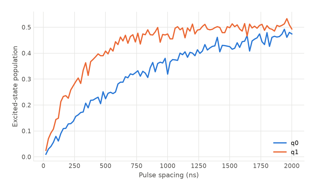
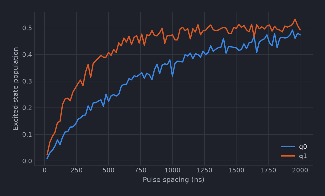
The total free evolution is four times the spacing, which is why the model reads 4 * env["tau"] rather than env["tau"]. The reference executor times nothing, so the wait operations contribute no duration of their own and that factor of four has to be written into the model by hand. On an instrument it would come out of the sequence.
Adapting it
To compare filter shapes rather than qubits, define a second fragment with a different train length and call both on the same qubit:
Because the length is structural, the two definitions both appear in the file and each call site names the one it wants. That is the honest form: a .qp reader can see how long each train is without evaluating anything.
A Hahn echo is this fragment with a train of one, and the T1 and Ramsey page introduces the pieces it is built from. Ramsey is the train of none.
To keep the IQ point alongside the population, add qp.MeasurementField.IQ to the fields= tuple inside the fragment. Everything the measurement records is decided at the definition, so a call site cannot ask for more, and a second kind of readout means a second fragment or a parameter that reaches the measurement.
To call the same fragment across a whole register, loop over the qubits at build time:
That writes eight call statements and one definition, and the handles come back as m0, m0_2 through m0_8 in call order after expand(). Reading eight records on one bus each is multiplexed readout territory, and the naming is what keeps them apart.