Rabi oscillation
Sweeping the drive amplitude on a qubit and reading it out at every amplitude gives the curve a pi-pulse amplitude is calibrated from. The program below is the smallest one that uses the pieces almost every experiment needs: an averaging block, one sweep, a pulse, a sync, and a measurement.
The program
import qprogram as qp

schema = qp.BusSchema.transmon()
q = schema.q

program = qp.QProgram(
    label="rabi",
    description="Rabi oscillation on q0",
    schema=schema,
)
gain = program.variable("gain", label="Drive amplitude", units="V")

with program.average(shots=1000):
    with program.sweep(gain, qp.Range(start=0.0, stop=1.0, step=0.01)):
        program.set_gain(q[0].drive, gain)
        program.play(q[0].drive, "pi_pulse")
        program.sync()
        m0 = program.measure(q[0].readout, "readout", "weights")

print(qp.dumps(program))
Why each piece is where it is
qp.BusSchema.transmon() declares one element, q, with two bus kinds: drive, which is IQ, and readout, which is IQ and has an ADC. The schema fixes no qubit count, so q[0] and q[7] both resolve, and the index appears only in the resolved bus string q0/drive. Calling measure on q[0].drive raises ValidationError: Bus 'q0/drive' does not support acquisition (acquires=False), because the check is against the acquires flag the schema records per bus kind.
qp.Range(start=0.0, stop=1.0, step=0.01) holds round((stop - start) / step) + 1 points, which is 101 here. A Range always starts at start and lands on stop only when the step divides the span evenly; qp.Range(0.0, 1.0, 0.3) ends at 0.9 instead. Use qp.Linspace(0.0, 1.0, num=101) when the last point has to land on stop whatever the arithmetic does.
The averaging block is outside the sweep, so the whole amplitude ramp runs 1000 times over rather than 1000 shots being taken at one amplitude before the next. Swapping the two with statements gives the other order and the same result shape, because an average block never contributes a result dimension; it decides only the order shots are taken in, which is what averages out drift between the first and the last point of the ramp.
set_gain scales the output of the drive bus, which is how the one "pi_pulse" envelope gets reused at all 101 amplitudes. Putting the variable inside the pulse instead is the other option, and the CZ chevron does that with its flux pulse: qp.waveforms.IQDrag(amplitude=gain, duration=40, sigma=8, beta=0.1) sweeps the envelope rather than the output stage. Which one a platform can compile is a capability question, not a language one.
program.sync() with no arguments aligns every bus the program has touched, so readout does not start before the drive pulse has finished. Pass a list to narrow it to those buses. Passing an empty list raises ValidationError, since sync([]) reads as either "sync nothing" or "sync everything".
measure returns the qp.MeasurementHandle that result.get takes later. Its name comes from the bus path plus a per-bus counter, so the first measurement on q0/readout is named q0/readout/m0. Handles compare by name rather than by identity, so a handle reconstructed after a .qp round-trip still finds the right record.
What it produces
qp.dumps(program) returns this, and it is the whole file:
#!QProgram 0.2

metadata:
  label: "rabi"
  description: "Rabi oscillation on q0"

schema:
  element q:
    drive info=IQ
    readout info=IQ+acquires

body:
  var gain label="Drive amplitude" units="V"

  average 1000:
    for gain in Range(start=0.0, stop=1.0, step=0.01):
      set_gain q[0].drive gain
      play q[0].drive "pi_pulse"
      sync
      measure q[0].readout "readout" "weights" name="q0/readout/m0"
The schema: block records the element and its bus kinds, not the qubits the program touched, which is why q[0] appears in the body but nowhere in the schema. Bus references are written as the compact q[0].drive path and resolve back through the schema on load. The writer spells out every sweep source argument by keyword and emits name= on every measurement even when the name was auto-allocated, so qp.loads(qp.dumps(program)) gets the same handle names back rather than reallocating them.
Plugging in calibration data
"pi_pulse", "readout", and "weights" are aliases. Resolving them produces a second program:
resolved = program.with_waveforms(
    {
        "pi_pulse": qp.waveforms.IQDrag(amplitude=0.5, duration=40, sigma=8, beta=0.1),
        "readout": qp.waveforms.IQPair(qp.waveforms.Square(1.0, 2000), qp.waveforms.Square(0.0, 2000)),
        "weights": qp.waveforms.IQPair(qp.waveforms.Square(1.0, 2000), qp.waveforms.Square(1.0, 2000)),
    }
)
The original program keeps its aliases; resolved is a deep copy with each matching name replaced. A name with no entry in the mapping passes through as a string, so a partial library is not an error. Each replacement re-runs the channel check, which is where an IQ pulse aimed at a single-channel bus is caught: ValidationError: Bus 'q0/flux' is a single channel but received an IQWaveform (IQPair).
A plain dict is one global tier, so "pi_pulse" resolves to the same pulse on every bus. Pass a qp.WaveformLibrary instead when a name has to mean different things on different qubits.
Running it
qp.simulate builds a throwaway qp.ReferencePlatform and executes on it. The result shapes are the ones a hardware platform's execute() has to produce as well, since vendor compilers are tested against what this executor returns:
result = qp.simulate(resolved)

data = result.get(m0)  # xarray.DataArray
data.dims  # ("gain", "IQ")
data.shape  # (101, 2)
data.coords["gain"]  # 0.00, 0.01, ..., 1.00
data.coords["IQ"]  # ["I", "Q"]
One dimension per enclosing sweep, named after the variable id and ordered outermost first, then a trailing "IQ" dimension of length 2. average is absent from the dims because the executor accumulates over shots and divides by the per-point shot count.
The reference executor runs no timing simulation: play, sync, and the bus-tuning operations (set_gain, set_frequency, set_phase, set_offset) evaluate their expressions and are otherwise no-ops. That is why passing the unresolved program here works too, and why with_waveforms is a requirement of hardware platforms rather than of qp.simulate.
It also means the IQ values are whatever the measurement model says. The default model responds 0j to everything, so data comes back as an array of exactly 0.0. Shape the response to see a curve:
import numpy as np

model = qp.MockMeasurementModel(
    response=lambda bus, env: np.sin(np.pi * env["gain"]) ** 2 + 0j,
    noise=0.02,
)
result = qp.simulate(resolved, model=model)
env holds the currently bound loop variables by id, plus the platform parameter store keyed "bus.parameter", so a response can depend on any of them. noise is the standard deviation of the gaussian added per quadrature per shot; the model draws from one seeded generator, so a fresh model on the same program gives the same numbers every time.
To get the raw ADC trace as well, ask for it where the measurement is built, by replacing the measure call in the program with this one:
m0 = program.measure(
    q[0].readout,
    "readout",
    "weights",
    fields=(qp.MeasurementField.IQ, qp.MeasurementField.RAW),
)
Then name the field when reading it back:
raw = result.get(m0, field=qp.MeasurementField.RAW)
raw.dims  # ("gain", "time", "IQ")
raw.shape  # (101, 16, 2)
result.get returns the IQ field unless another one is named, and asking for a field the measurement did not request raises KeyError: Measurement 'q0/readout/m0' has no field 'state'; available: iq, raw rather than substituting a different array. The 16 time samples are the default of MockMeasurementModel's raw_samples argument, which a real ADC record would replace.
Plotting
Plotting needs matplotlib, which is not a runtime dependency of the package. It comes with the viz extra:
result.plot works the figure out from the array's shape. One swept dimension besides IQ gives a line per quadrature:
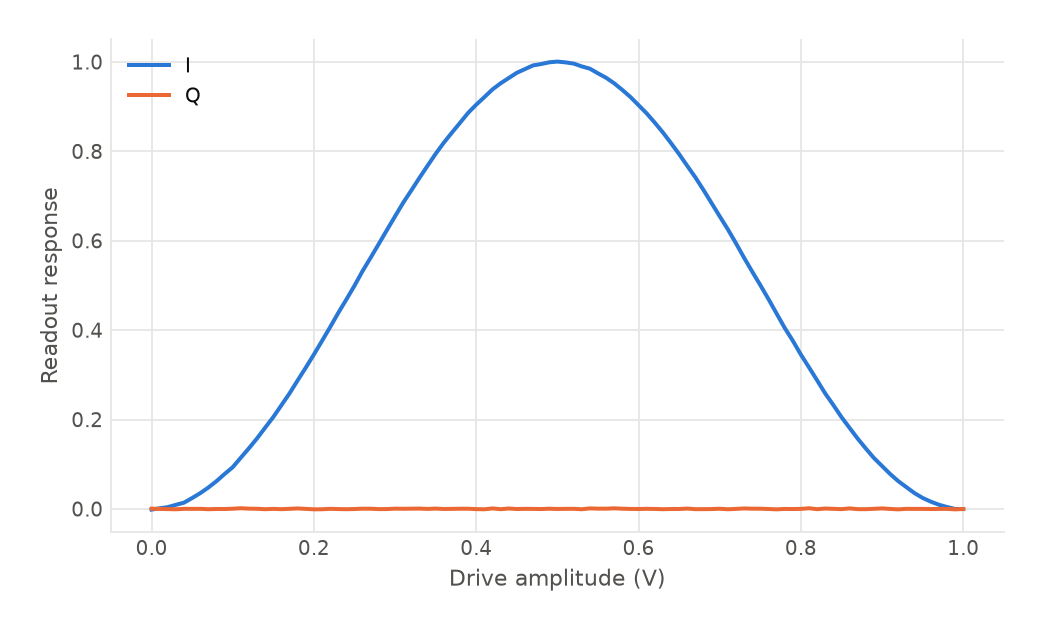
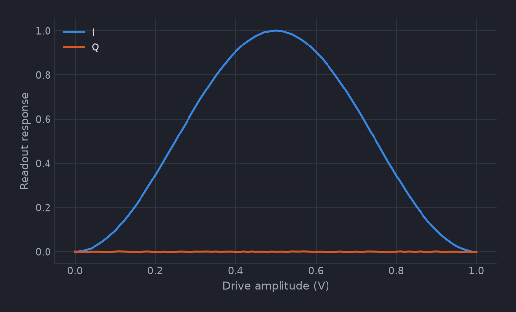
Nothing about the x axis is typed out. The label and units given to program.variable reach the coordinate as its long_name and units attributes, and the axis reads them:
value= is there because the other axis has no such source: what a demodulated point means is the readout chain's business, not the program's. A qp.plotting.Quantity is also how a coordinate gets restated for the figure, in the units you want to read it in. The call returns the matplotlib Axes, so anything else the figure does not decide is a method away on it. Plotting results has the rest: heatmaps and scatters, the channels argument, themes, and registering a renderer of your own.
Adapting it
For a chip that is not a fixed-frequency transmon, change the schema. The presets are qp.BusSchema.transmon, transmon_coupled, flux_tunable_transmon, flux_tunable_transmon_coupled, fluxonium, and fluxonium_coupled; BusSchema.add_element builds one at runtime, and subclassing BusSchema gives typed accessors. See Buses and schemas.
To sweep frequency as well, add program.set_frequency(q[0].drive, freq) and a second sweep. Nesting the two gives the full grid and a two-dimensional result; composing them with | advances them in lockstep and gives one "gain|freq" dimension carrying both coordinates, which plot draws as one axis and a twin axis above it. Both loops must then have the same length. See Control flow.
To read the classified state instead of the IQ point, request fields=(qp.MeasurementField.STATE,) and read result.get(m0, field=qp.MeasurementField.STATE), which has the sweep dims and no trailing "IQ". Under averaging it holds the excited-state population rather than a single 0 or 1. See Measurements and results.