Qubit spectroscopy
The frequency a qubit answers to is the first number an experiment needs, and finding it is a frequency sweep. Park a long, weak tone on the drive bus, step its frequency across a window, and read the qubit out at every step. Where the tone lands on the transition the qubit is driven out of its ground state and the readout response moves with it, so the feature that appears in the sweep locates f01. Everything the Rabi example does starts here, because the "pi_pulse" alias it plays only means something once this measurement has found the frequency to play it at.
Two things appear here that the Rabi program does not have: the swept quantity reaches the instrument through set_frequency rather than through a gain or a waveform parameter, and the sweep is a qp.Linspace rather than a qp.Range. The control flow is unchanged, so the whole difference between the two experiments is which operation the loop variable feeds.
The program
import qprogram as qp

schema = qp.BusSchema.transmon()
q = schema.q

program = qp.QProgram(
    label="qubit_spectroscopy",
    description="Two-tone spectroscopy of q0",
    schema=schema,
)
freq = program.variable("freq", label="Drive frequency", units="Hz")

with program.average(shots=1000):
    with program.sweep(freq, qp.Linspace(4.6e9, 5.4e9, num=201)):
        program.set_frequency(q[0].drive, freq)
        program.play(q[0].drive, "saturation")
        program.sync()
        m0 = program.measure(q[0].readout, "readout", "weights")
Why each piece is where it is
set_frequency retunes the oscillator on a bus and takes its argument in Hz. It accepts a plain float or an Expression, which is what lets the loop variable go straight in: the sweep binds freq to a new value at each iteration and the operation writes that value to the drive NCO. The operation is a leaf like any other, so it sits in the loop body next to the play it affects rather than being configuration attached to the bus.
qp.Linspace(4.6e9, 5.4e9, num=201) gives 201 points with both ends included. A spectroscopy window is described by its edges and by how many points you can afford across them, which is exactly the two things Linspace takes; it derives the spacing, and Linspace(4.6e9, 5.4e9, num=201).step() reports the 4 MHz it arrived at. qp.Range takes the other pair, a start and a spacing, and derives the count and the last point, which lands on stop only when the step divides the span evenly. Either is usable here, and the choice is about which two numbers you actually know.
Both sources are KIND "linear", so a platform is free to compile either as a hardware ramp over one register rather than as a table of 201 values. Writing the same 201 points as qp.Values gives up that option: Values is KIND "arbitrary" even when its points are evenly spaced, because the source proves nothing about their regularity to a compiler. See Capabilities, diagnostics, and profiles for how a platform declares which kinds it can take.
"saturation" is a long, weak pulse, and both halves of that matter on hardware. Long, because a tone of 20 microseconds has a bandwidth far narrower than the 4 MHz step, so it interrogates one point of the window at a time rather than smearing across several. Weak, because a strong tone power-broadens the transition and pulls it, which widens the feature and moves the center away from the frequency you are trying to measure. The reference executor renders no envelope, so neither effect appears in the run below; they are the reason the alias resolves to the pulse it does on an instrument.
The average block sits outside the sweep, so the whole window is scanned 1000 times over rather than 1000 shots being taken at one frequency before moving on. sync() with no arguments aligns every bus the program has touched, which here keeps the readout from starting before the saturation tone has finished. Both are the same decisions the Rabi example explains at length.
What it produces
#!QProgram 0.2

metadata:
  label: "qubit_spectroscopy"
  description: "Two-tone spectroscopy of q0"

schema:
  element q:
    drive info=IQ
    readout info=IQ+acquires

body:
  var freq label="Drive frequency" units="Hz"

  average 1000:
    for freq in Linspace(start=4600000000.0, stop=5400000000.0, num=201):
      set_frequency q[0].drive freq
      play q[0].drive "saturation"
      sync
      measure q[0].readout "readout" "weights" name="q0/readout/m0"
The sweep source is written with every argument named, so a reader of the file does not have to know the constructor's positional order, and the bounds come back as floats because a source stores them that way. set_frequency writes its argument as the bare identifier freq, which the parser resolves against the var declaration above it.
Running it
The three aliases resolve against a calibration set, and qp.simulate runs the resolved copy on the reference platform:
import numpy as np

library = {
    "saturation": qp.waveforms.IQPair(qp.waveforms.Square(0.02, 20000), qp.waveforms.Square(0.0, 20000)),
    "readout": qp.waveforms.IQPair(qp.waveforms.Square(1.0, 2000), qp.waveforms.Square(0.0, 2000)),
    "weights": qp.waveforms.IQPair(qp.waveforms.Square(1.0, 2000), qp.waveforms.Square(1.0, 2000)),
}


def lorentzian(bus, env):
    """A saturated transition: unit height at 5 GHz, 8 MHz half width."""
    f0, hwhm = 5.0e9, 8e6
    return 1.0 / (1.0 + ((env["freq"] - f0) / hwhm) ** 2) + 0j


result = qp.simulate(
    program.with_waveforms(library),
    model=qp.MockMeasurementModel(response=lorentzian, noise=0.01),
)

data = result.get(m0)
data.dims  # ("freq", "IQ")
data.shape  # (201, 2)
data.coords["freq"]  # 4.600e9, 4.604e9, ..., 5.400e9
One dimension for the sweep and a trailing "IQ" dimension of length 2, the same shape the Rabi program returns, since the two have the same control flow.
The peak is the model's, not the executor's. set_frequency evaluates its expression and is otherwise a no-op, exactly as play and sync are, so nothing in the run knows what a qubit is. What produces the curve is lorentzian reading env["freq"], which holds the loop variable bound at the grid point being measured. Without a model= argument every value comes back as 0.0.
Plotting
Spectroscopy is usually read as a magnitude rather than as two quadratures, since the phase of the transmitted signal depends on cable length and the feature does not:
result.plot(
    m0,
    channels="magnitude",
    coords={"freq": qp.plotting.Quantity(units="GHz", transform=lambda v: v / 1e9)},
    value=qp.plotting.Quantity("Readout magnitude"),
)
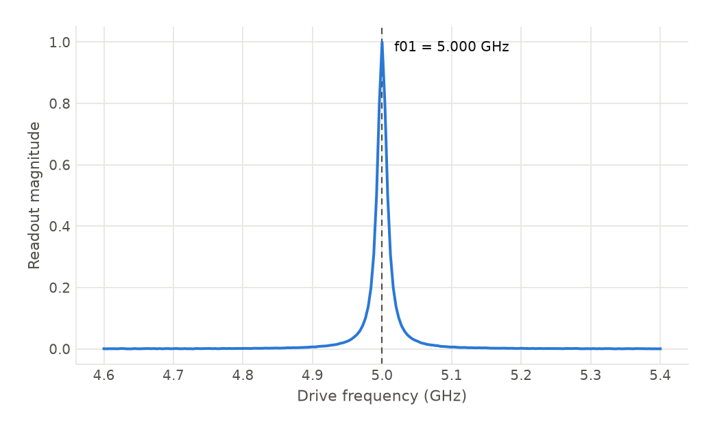
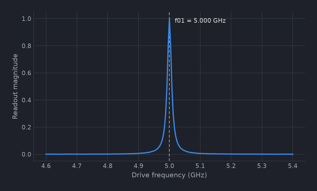
channels="magnitude" is np.hypot(I, Q), and the qp.plotting.Quantity on coords restates the axis in gigahertz: the arithmetic and the unit it produces travel as one object, so the axis cannot end up reading (Hz) over numbers running 4.6 to 5.4. matplotlib is not a runtime dependency; it comes with the viz extra, installed with pip install "qprogram[viz]".
The figure is restated; the result is not. Reading the peak back is arithmetic on the array, and the array is still in hertz:
magnitude = np.hypot(data.sel(IQ="I"), data.sel(IQ="Q"))
f01 = float(data.coords["freq"][int(np.argmax(magnitude.values))])  # 5.0e9
np.hypot over two sel results returns a DataArray with dims ("freq",), so the coordinate survives the arithmetic and the peak comes back as a frequency. np.argmax wants the underlying array rather than the DataArray, which is what .values is for; handing it the labelled array raises ValueError: dimensions ('freq',) must have the same length as the number of data dimensions, ndim=0. The same split is worth remembering for anything you draw on the axes plot returns: they are in the figure's units, so marking the peak is ax.axvline(f01 / 1e9).
Adapting it
The scan above is the coarse one. Once it has put f01 near 5 GHz, the next measurement is a narrow window centered there, and the natural way to write it is to sweep the detuning and add the center in the program:
fine = qp.QProgram(label="qubit_spectroscopy_fine", schema=schema)
det = fine.variable("det", label="Detuning", units="Hz")

with fine.average(shots=1000):
    with fine.sweep(det, qp.Linspace(-20e6, 20e6, num=161)):
        fine.set_frequency(q[0].drive, 5.0e9 + det)
        fine.play(q[0].drive, "saturation")
        fine.sync()
        m = fine.measure(q[0].readout, "readout", "weights")
5.0e9 + det is the first expression on these pages that is not a bare variable, and it serializes as one:
The addition survives into the file because one of its operands is a variable the program will not know a value for until it runs. Arithmetic between plain numbers does not: Python evaluates 2 * np.pi * 2e-3 before the DSL is handed the result, so only the part that touches a variable becomes a node. The cost of the node is a wider capability requirement. set_frequency with a bare variable asks a platform for op.set_frequency and expr.variable; with the sum it also asks for expr.binary_op and expr.constant, which a sequencer that can only load a swept register into a frequency word cannot supply. See Variables and expressions.
To measure how hard the tone is driving the transition, put an amplitude sweep outside the frequency sweep and use set_gain. The peak broadens and shifts with power, and the two-dimensional result that comes back is read the same way the CZ chevron reads its grid.
For a window that is dense near the peak and coarse away from it, pass the points explicitly with qp.Values, at the cost of the "linear" kind and whatever a platform does with it:
points = np.concatenate(
    [np.arange(4.6e9, 4.95e9, 10e6), np.arange(4.95e9, 5.05e9, 1e6), np.arange(5.05e9, 5.4e9, 10e6)]
)
with program.sweep(freq, qp.Values(points)):
    ...
To find the readout resonator rather than the qubit, the swept knob is usually the local oscillator feeding the readout line rather than an NCO the sequencer owns, which makes it a set_parameter and moves the sweep host-side. See Running programs.