Single-shot readout
Averaging is what every other page here does, and it is what hides the question this one asks. A Rabi curve at 0.5 excited population is the same curve whether each shot lands cleanly in one of two blobs or whether the two blobs overlap so badly that half the classifications are guesses. Telling those apart means keeping the shots: prepare the ground state a few thousand times, prepare the excited state a few thousand times, and look at where the individual points land.
This is the only program in this section with no average block. That one absence changes how the result is shaped, forces the shot index to be something the program says out loud, and makes the measurement model worth writing by hand rather than reaching for qp.MockMeasurementModel.
The program
import numpy as np
import qprogram as qp

schema = qp.BusSchema.transmon()
q = schema.q

program = qp.QProgram(
    label="single_shot_readout",
    description="Ground and excited shots, unaveraged",
    schema=schema,
)
prepared = program.variable("prepared", label="Prepared state")
shot = program.variable("shot", label="Shot index")

with program.sweep(prepared, qp.Values([0, 1])):
    with program.sweep(shot, qp.Range(0, 1999, 1)):
        program.set_gain(q[0].drive, prepared)
        program.play(q[0].drive, "pi_pulse")
        program.sync()
        shots = program.measure(
            q[0].readout,
            "readout",
            "weights",
            fields=(qp.MeasurementField.IQ, qp.MeasurementField.STATE),
            name="shots",
        )
Why each piece is where it is
Only a sweep contributes a result dimension. An average block deliberately does not, since its whole job is to collapse the shots it encloses, and neither does a plain block or a conditional. So a program that wants to keep its shots cannot use average at all, and the shot index has to be a real sweep.
That is the awkward part of this page and worth naming rather than hiding. shot is a variable no operation ever reads. It exists to give the inner loop something to bind so that the loop contributes an axis, and it lands in the file as a var declaration and a 2000-point ramp that a compiler has to treat as a real value table. Nothing objects to it: qp.validate returns no diagnostics and the run emits no warning.
prepared earns its keep, though. qp.Values([0, 1]) is a two-point categorical axis rather than a ramp, and set_gain(q[0].drive, prepared) turns it into the preparation: at 0 the drive output is scaled to nothing and the "pi_pulse" leaves the qubit in the ground state, at 1 it plays at full amplitude and inverts it. One pulse, one gain, two preparations.
The measurement is given an explicit name="shots" rather than taking the auto-allocated q0/readout/m0. With one measurement in the program the name is a convenience, but it is the name the result is read back by, and a name that says what the record is survives refactoring better than a positional one.
Nesting order matters here in a way it does not around an average. The outer sweep becomes the first dimension, so swapping the two with statements transposes the result from (2, 2000) to (2000, 2) rather than being free.
What it produces
#!QProgram 0.2

metadata:
  label: "single_shot_readout"
  description: "Ground and excited shots, unaveraged"

schema:
  element q:
    drive info=IQ
    readout info=IQ+acquires

body:
  var prepared label="Prepared state"
  var shot label="Shot index"

  for prepared in [0.0, 1.0]:
    for shot in Range(start=0.0, stop=1999.0, step=1.0):
      set_gain q[0].drive prepared
      play q[0].drive "pi_pulse"
      sync
      measure q[0].readout "readout" "weights" name="shots" fields=["state", "iq"]
qp.Values writes as the bare list [0.0, 1.0], which is the format's sugar for it, and the integers become floats because a sweep source stores its points that way. The explicit name appears in name= exactly as the auto-allocated ones do on every other page, since the writer emits the attribute either way.
Writing a measurement model
qp.MockMeasurementModel puts every shot at one point and adds noise around it, which is the right model for a curve and the wrong one for a blob. What this page needs is a model where the classified state is a function of where the shot actually landed, so that misclassification is something the run produces rather than something imposed on it.
qp.MeasurementModel is a protocol with one method:
class ReadoutModel:
    """Two gaussian blobs in the IQ plane, classified by a threshold on I."""

    def __init__(self, separation=4.0, sigma=1.0, seed=0):
        self.separation = separation
        self.sigma = sigma
        self._rng = np.random.default_rng(seed)

    def sample(self, bus, env):
        center = self.separation if env["prepared"] else 0.0
        i = center + self._rng.normal(0.0, self.sigma)
        qv = self._rng.normal(0.0, self.sigma)
        return qp.MeasurementSample(i=i, q=qv, state=int(i > self.separation / 2))
sample receives the bus string and the environment, which holds the bound loop variables by id plus any platform parameters. It does not receive the measurement's name, so a model cannot answer two measurements on the same bus differently; where that matters, the distinction has to come through env.
qp.MeasurementSample carries four fields, of which only i, q, and state have to be given. raw defaults to an empty (0, 2) array, which is what a model with no ADC to simulate wants, and it is read only by a measurement that requests MeasurementField.RAW. Asking for that field from this model raises, naming the shape it got and the shape it wanted, rather than broadcasting the empty trace into the accumulator. Declaring raw_samples on the model and returning a trace of shape (raw_samples, 2) is what makes the field available.
The threshold at half the separation is what makes the state a classification rather than a label: a ground-state shot that scatters past it is recorded as excited, which is exactly the error the experiment measures.
Reading the shots
library = {
    "pi_pulse": qp.waveforms.IQDrag(0.5, 40, 8, 0.1),
    "readout": qp.waveforms.IQPair(qp.waveforms.Square(1.0, 2000), qp.waveforms.Square(0.0, 2000)),
    "weights": qp.waveforms.IQPair(qp.waveforms.Square(1.0, 2000), qp.waveforms.Square(1.0, 2000)),
}

result = qp.simulate(program.with_waveforms(library), model=ReadoutModel(seed=0))

iq = result.get(shots)
iq.dims  # ("prepared", "shot", "IQ")
iq.shape  # (2, 2000, 2)

state = result.get("shots", field=qp.MeasurementField.STATE)
state.dims  # ("prepared", "shot")
state.shape  # (2, 2000)
Three dimensions where the other pages have two, and the middle one is the shot. Nothing was averaged: each entry is one measurement of one shot, because the executor divides by a per-point shot count that is 1 everywhere here.
The two error rates and the fidelity fall straight out of the state array:
v = state.values
false_excited = v[0].mean()  # 0.02
true_excited = v[1].mean()  # 0.975
fidelity = 1 - (false_excited + (1 - true_excited)) / 2  # 0.9775
The state field is float64, not an integer, because it goes through the same divide-by-shot-count path as everything else even when that count is 1. The values are exactly 0.0 and 1.0 so comparisons work, but v[1, 0] is 1 is False, and anything that wants an index or a bin count needs .astype(int) first.
Plotting the two blobs is what the page is for, and the IQ array is already laid out for it:
import matplotlib.pyplot as plt

plt.scatter(iq[0].sel(IQ="I"), iq[0].sel(IQ="Q"), s=2, label="prepared |0>")
plt.scatter(iq[1].sel(IQ="I"), iq[1].sel(IQ="Q"), s=2, label="prepared |1>")
plt.axvline(2.0, color="k", lw=0.5)  # the classifier threshold
plt.legend()
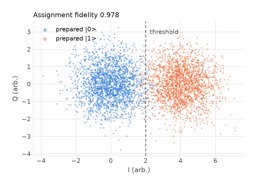
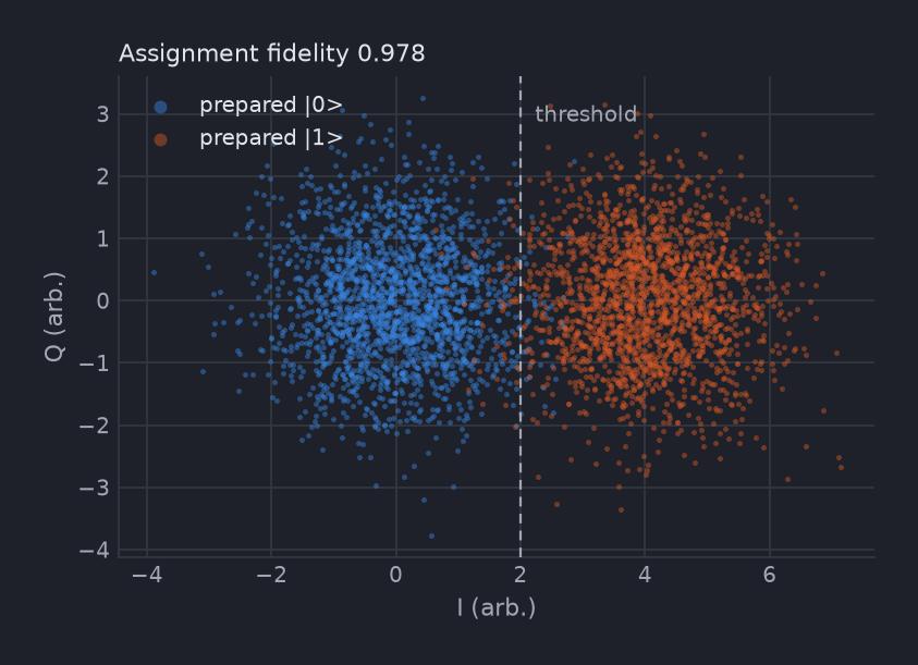
result.plot(shots, kind="scatter") draws the same plane in one call, but as a single cloud: two colours by prepared state and a line at the threshold are a layout, and nothing on the result says those three things belong in one figure. Plotting results draws the line between what plot infers and what stays here.
Four thousand shots run in well under a tenth of a second, so this is the cheapest program in the section despite having the most records. The combination to be careful with is not the shot count but the shot count times MeasurementField.RAW, which allocates a trace per shot rather than per averaged point.
Adapting it
To find the threshold rather than assume it, drop MeasurementField.STATE and classify the IQ array yourself. The state field is whatever the model or the instrument decided; the I and Q values are the evidence, and fitting two gaussians to them is what produces a threshold in the first place. On hardware this is the ordering that matters, since the discriminator has to be calibrated before it can be trusted.
To see how few dimensions a result can have, take the sweeps away. A measurement with no enclosing loop at all gives a scalar:
result.get(handle, field=qp.MeasurementField.STATE).dims  # ()
result.get(handle, field=qp.MeasurementField.STATE).shape  # ()
That is the floor: one number, no axes. Asking the same measurement for IQ gives ("IQ",) and shape (2,), since the quadrature pair is a dimension the field carries rather than one a loop produced.
qp.Repeat looks like a way to get shots without the unused variable and is not. It multiplies a source's points instead of adding an axis:
with program.sweep(prepared, qp.Repeat(qp.Values([0, 1]), times=4)):
    ...
# dims ("prepared",), shape (8,), coords [0. 1. 0. 1. 0. 1. 0. 1.]
One flattened axis with repeated coordinates, which is a different thing from a shot dimension and gives you no way to select a single repetition. If you want the shots separated, the inner sweep is the way.
To measure a whole register single-shot, add the other qubits' measurements inside the same loop the way multiplexed readout does. Correlations between qubits are visible only in unaveraged data, so the two ideas belong together: averaging each qubit separately destroys exactly the joint information a parity check needs.